 Study Plan
2110 Topo
Study Plan
2110 Topo
ST 2110-21: Traffic Shaping & Buffer Models
ST 2110-21 defines how senders must pace packets and how much buffering receivers and switches must provide to handle timing variations in uncompressed video streams.
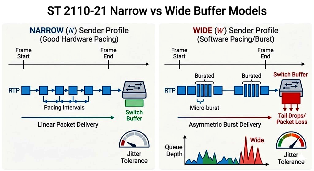
This micro-burst is catastrophic for a switch. The packets arrive so fast that they fill the internal hardware buffer for that output port almost instantly. Once the buffer is full, the switch must drop all subsequent packets until the buffer has been serviced (tail-drops). The "Narrow" sender model uses hardware pacing to deliver packets uniformly, ensuring the switch buffer is never overwhelmed and the stream remains deterministi
 This page establishes that the only way to meet strict linear pacing requirements is with hardware. This second graphic moves the discussion inside the endpoint device. It shows that both the mandatory Narrow (N) and Narrow Linear (NL) profiles rely on a high-precision, dedicated clock on the Network Interface Card (NIC) to manage packet egress. The Hardware Pacing path uses a dedicated clock (like a T-GIE or a PLL) to meter packets onto the wire with perfect spacing, matching the theoretical Narrow model.
Conversely, the Software Pacing path shows what happens on systems that lack this hardware: the system CPU and the non-real-time Operating System attempt to pace the packets in software. This path introduces inevitable operating system jitter, resulting in the irregular, Bursty packet delivery characteristic of the Profile W (Wide) model. This is why "Wide" streams require the switch to maintain significantly larger buffers to accommodate the CPU's unpredictable nature.
Key Concepts a 2110 Designer Must Know
Why Pacing is the Most Critical Factor in ST 2110
Uncompressed ST 2110-20 video produces extremely high, constant bitrates — often 1.5 Gbps to over 12 Gbps per stream — with very large packets. Because there is no compression to smooth the data, the sender must carefully control when each packet is transmitted. This controlled transmission is called pacing, as defined in ST 2110-21.
What Proper Pacing Achieves
- Sends packets at a smooth, predictable rate instead of in large, sudden bursts.
- Prevents overwhelming switch output queues.
- Reduces the risk of buffer overflow and packet loss.
- Allows the network to handle multiple high-bandwidth flows reliably.
The Fundamental Difference Between Narrow (N) and Wide (W) Senders in ST 2110-21
The core distinction between a Narrow sender and a Wide sender lies in how much they rely on the network switch’s buffering capability.
Narrow (N) Sender
- Very strict, tight packet pacing
- Sends packets in a highly uniform, evenly spaced manner
- Requires very little buffering from the switches
- Places most timing responsibility on the sender
- More demanding on sender hardware
- Easier on the network fabric
Preferred for most professional live broadcast environments.
Wide (W) Sender
- More relaxed pacing
- Allows larger bursts of packets
- Relies heavily on switch buffer depth
- Places more responsibility on the network hardware
- Easier on sender hardware
- More demanding on the network
Requires switches with deeper output buffers to absorb bursts.
Additional Notes: W is typically for legacy equipment or specific software-defined senders that cannot achieve hardware-level pacing; it explicitly warns against using it for core infrastructure where switch buffer predictability is required.
In addition if a device does not have a dedicated hardware clock, the system CPU and non-real-time OS generate "jitter" in packet release, making it physically impossible to maintain the rigid, microsecond-accurate intervals required by the Narrow (N) profile.
A sender must declare its profile (N, NL, W) within the SDP (Session Description Protocol) file. The receiver and the network controller use this information to determine if the stream is "safe" to join and to allocate the necessary buffer depth required to play the stream back without stuttering.
A Narrow sender is “well-behaved” and needs minimal help from the network. A Wide sender is “burstier” and depends on the switches having large enough buffers to smooth out the traffic. Most professional 2110 facilities prefer Narrow senders because they are more predictable and put less stress on the network fabric.
The Primary Consequence of Poor Pacing
If a sender fails to pace its packets correctly, it transmits them in large, uncontrolled bursts.
The main result is switch buffer overflow:
- Switch output queues fill faster than they can be drained.
- Once the buffer is full, the switch begins dropping packets (tail drop).
- This leads to visible video artifacts, dropped frames, freezing, or complete loss of signal at the receiver.
In uncompressed ST 2110 systems, pacing is not optional — it is the primary mechanism that prevents the massive video streams from overwhelming the network fabric. Even the best switches and QoS configurations will fail if senders do not properly pace their packets.
1. Sender Traffic Shaping (Pacing Profiles)
- Narrow Profile: Strictest pacing. Packets are sent very evenly. Lowest risk of congestion. Most common in live production.
- Wide Profile: More tolerant of bursts. Easier on some hardware but requires larger buffers.
2. Buffer Models
2110-21 defines two main receiver buffer models:
- Narrow Buffer Model: Smaller buffer size. Requires very precise sender pacing. Lower latency.
- Narrow Senders are usually FPGA-based and are highly precise, adding a very minimal delay or jitter to the resulting IP stream.
- Narrow Senders can be divided into two sub-categories, namely Narrow Linear Senders (type NL) and Narrow Gapped Senders (type N - the "gapped" part is implied).
- Narrow Senders adhere much more tightly to narrow timing constraints, while Wide Senders can vary more widely in their packet pacing.
- Narrow Linear - Senders space out the packets evenly.
- Wide Buffer Model: Larger buffer. More tolerant of network jitter and sender behavior. Higher latency.
- A Wide Sender can comprise a regular PC with some dedicated hardware that makes it capable of handling uncompressed video. Even with the dedicated hardware however, the transmitting PC can struggle to output packets at a steady pace. This variability in the rate of transmission places greater demands on the Receiver in terms of the buffering and memory required. As such, if there is a Wide Sender anywhere in your network, you will need a corresponding Wide Receiver.
3. Design Implications
- Switches must have deep enough buffers on output queues.
- Proper QoS (CS5/AF41 for video) is essential.
- End-to-end MTU must be consistent (usually 9000+).
- Most facilities design around the Narrow profile for best performance.
ST 2110-21 is the “traffic discipline” standard. Choose your buffer model carefully — Narrow gives better performance but is less forgiving, while Wide is more robust but adds latency. Most professional live facilities standardize on Narrow pacing with proper QoS and buffer sizing.
Testing Methodology for ST 2110-21 Compliance
ST 2110-21 defines strict traffic shaping and buffer requirements for uncompressed video. Testing should evaluate how well the system handles real-world network impairments.
Key Impairments to Test
- Delay
Caused by physical link length or processing delays in network elements. Constant delay is usually not an issue (as long as it is within reason). Variable delay (especially packet-by-packet) should be tested from 20 µs up to several milliseconds to verify the receiver’s re-alignment capability. - Packet Loss
Typically caused by congestion or corruption. Receivers using ST 2022-7 Seamless Protection Switching should tolerate significant packet loss on one path. Test both with and without 2022-7 enabled. - Packet Corruption
Often caused by dirty fiber, bad connections, or EMI. Cut-through switches do not perform CRC checks, so corrupted packets may be forwarded. The receiver’s MAC layer should drop them. Test correlation between introduced corruption and observed packet loss. - Bursty Conditions
Large bursts of packets can overwhelm receiver buffers. Use burst impairment tools (e.g., Calnex SNE Burst mode) to verify that your chosen buffer model (Narrow or Wide) is sufficient. If the sender is "Wide" (bursty), it can saturate a switch port buffer even on a low-load link, causing drops. That is even if the link showing only 40% bandwidth utilization. - Packet Reordering
Rare on well-designed LANs, but more common over WANs with multiple paths. Receivers must be able to reorder packets based on RTP sequence numbers. - Packet Duplication
Can occur due to misconfiguration (e.g., duplicate multicast streams) or network loops. Receivers should gracefully handle duplicates. - Jitter & Packet Delay Variation (PDV)
Introduced when packets pass through multiple routers/switches with varying queue depths. This is one of the most important impairments to test, as excessive jitter can cause buffer underruns or overruns.
If the SDI video output starts to flicker or show artifacts during impairment testing, it usually indicates that the receiver’s buffer size is too small for the applied jitter or burst conditions. Increasing the buffer depth (if adjustable) often resolves the issue.
The Virtual Receiver Buffer Model (VRB) in ST 2110-21
The Virtual Receiver Buffer Model (VRB) is a mathematical model defined in ST 2110-21 that acts as a safety check for engineers designing 2110 networks.
What is the VRB?
It is a virtual (simulated) buffer that represents the minimum buffering capability a compliant receiver must have. It calculates how much timing variation (jitter) and delay a stream can experience before the receiver’s buffer would overflow or underflow.
How the VRB Acts as a Safety Check
- Verifies Sender Compliance: It ensures the sender’s packet pacing (Narrow or Wide) stays within acceptable limits.
- Tests Network Design: It helps determine whether the real network (switches, links, QoS settings) will introduce too much jitter or delay for the chosen buffer model.
- Predicts Stability: If a stream stays within the VRB limits, the real receiver should be able to play the video cleanly without buffer underruns or overruns.
- Guides Buffer Sizing: It tells the engineer how large the receiver’s buffer needs to be for reliable operation.
Practical Use for Designers
When designing a 2110 system, engineers use the VRB as a benchmark:
- They test the actual network under load and measure packet arrival timing.
- They feed this timing data into the VRB model.
- If the model shows the buffer stays within safe limits, the design is considered safe.
- If the VRB shows frequent buffer violations, the engineer knows they must improve pacing, QoS, or switch buffering.
The Virtual Receiver Buffer Model is the engineer’s “stress test” tool. It provides a standardized way to predict whether the network will be stable for uncompressed video before the system goes live. A well-designed 2110 network should keep traffic comfortably within the VRB limits for the chosen Narrow or Wide profile.
How to Implement and Use the Virtual Receiver Buffer Model (VRB)
The Virtual Receiver Buffer Model (VRB) is a simulation tool defined in ST 2110-21. It allows engineers to predict whether their network design will support stable uncompressed video before going live.
Practical Implementation Steps
- Capture Real Network Traffic
Use a high-precision packet capture tool (e.g., Calnex SNE, Spirent, or Wireshark with hardware timestamping) on the receiver port. Capture under normal and stressed load conditions. - Measure Key Timing Parameters
Analyze the capture to determine:- Packet inter-arrival time (jitter)
- Maximum burst size
- Packet delay variation (PDV)
- Apply the VRB Model
Feed the measured timing data into the VRB mathematical model (many test tools have built-in VRB calculators). The model simulates how a compliant receiver’s buffer would behave. - Evaluate Results
Check whether the simulated buffer stays within safe limits:- No buffer underruns (starvation)
- No buffer overflows
- Iterate if Needed
If the VRB shows violations, improve the design by:- Tightening sender pacing (Narrow profile)
- Improving QoS configuration
- Adding deeper buffers on switches
- Reducing network hops or congestion
Tools Commonly Used
- Calnex SNE / Paragon (has built-in VRB analysis)
- Spirent TestCenter or Novus
- Wireshark + custom analysis scripts
The VRB is your virtual stress test. By measuring real packet timing and running it through the VRB model, you can predict whether your network will reliably support ST 2110-20 video before you deploy it. A clean VRB result gives you high confidence in your design.